Originally this was going to be one entry - but it started to get very long and so I decided it best to split it down: Part 1 covers the fundamentals of building the neural network; Part 2 will look at using what I have built and have a bit of fun with experimentation.
I’ve tried to cover as much as I can of what I’ve learned and discovered over the course of my implementation of this, but really this is just scratching the surface of what I could reasonably fit on this page. If you just want to see the code, the full source is available on github. I’m sticking to the basics here and trying to avoid getting too deep into the weeds of mathematical computations and keep the focus on the implementation / engineering as that’s ultimately what I know best.
Why Build from Scratch?
I’ll be honest - when I first started looking into machine learning everything felt very abstract, there were terms thrown around all over the place that I didn’t truly understand. Is the gradient descent a degenerative condition? Should one seeking medical advice before using a back prop? I could just ignore all this, whip out PyTorch and move on, but I wanted to really get a feel for what was going on inside.
So here we are, implementing it. I’ve chosen Rust for this - it’s a language I like the principles of, and I’m currently more familiar with than Python (which would be the obvious choice in the world of ML). Having said that, over the course of my explorations I hope to do a bit of both here and there.
The Big Picture - A Neural Network
The first thing to address is what I’m trying to build. I think it’s important to have a decent understanding of what the end goal is, so I can better see where the pieces fit as I build them from the ground up.
Neural networks are based on the principles of the human central nervous system - a network of neurons which, put simply, turn on and off to send signals around the body. If I use the analogy of touch, your finger touches a flame (the input), this signal is passed from neuron to neuron until eventually it reaches the brain and the result is to trigger pain. It’s a similar idea here - in much the same was as you would teach a child not to play with fire, I first need to teach my network what pain is (ok, maybe not the same way). Once it understands pain, I can then use it to test other inputs and determine if they are also painful or not. This is Supervised Learning, there are other methods to train networks which I might explore at a later date.
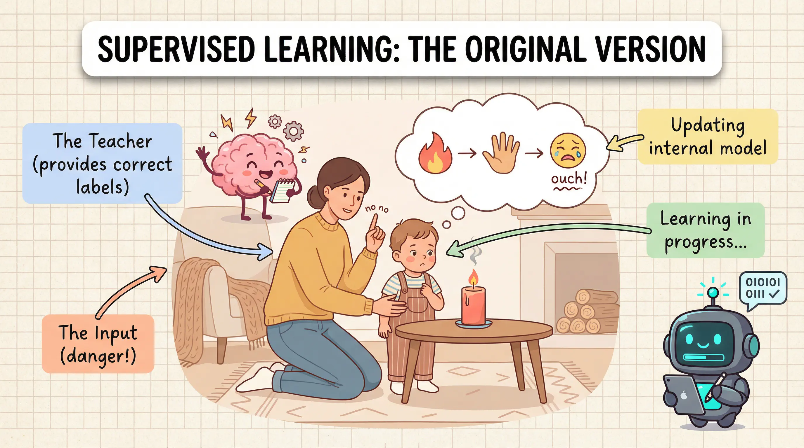
Supervised learning: the original version
But why bother? Surely you could program some simple logic: if temperature > 40 then pain; well that could work… for that case at least, but what about when you get stung by a bee? Ok, add that logic too, how about different pain thresholds? - eventually you will see this is a near impossible task to cover all possible scenarios reliably. That’s where machine learning really shines because I don’t need to teach it everything but just enough to understand what is expected from certain inputs. But look, I’m already getting over excited so I’ll get on with the implementation, and I’ll explore this more in Part 2 with some experimentation!
The XOR Problem
Well first let’s just set some expectations; this isn’t the frontier of machine learning development. To keep this comprehendable I’m going to train the network to understand XOR logic. This is actually an interesting problem to solve, because there was a point in time that it was thought impossible for a neural network to solve; and in fact, as I understand it, it is still impossible for a single-layer network to solve. This implementation will require multiple layers within the network.
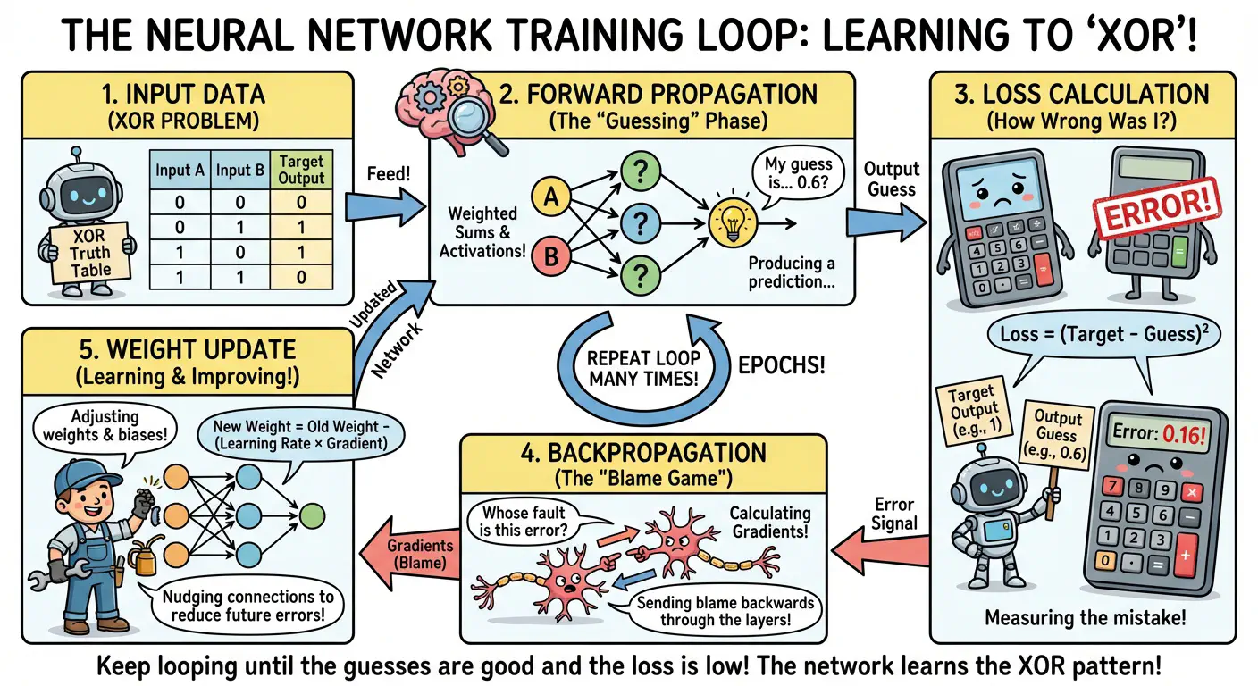
1. Input
This is the data that’s going to be fed into the network in order to train it. For the XOR problem, each piece of training data has two parts: the features (the actual inputs - in our case, two values A and B) and the target (what I want the network to output for those inputs).
For XOR specifically, there are four training examples: [0,0]→0, [0,1]→1, [1,0]→1, and [1,1]→0. The network doesn’t know the XOR pattern yet - it’s starting with random weights. The network needs to review these examples repeatedly until it figures out the pattern.
2. Forward Pass
The network pushes input data through, one layer at a time. Each layer takes the data it receives, multiplies it by its weights (think of these as the layer’s “settings”), adds a bias, and then applies an activation function to produce an output. That output becomes the input for the next layer.
This is called the “forward” pass because data moves forward through the network from input to output. For the XOR example, I might feed in [0, 1], and after passing through the hidden layer and output layer, the network spits out a prediction - maybe 0.58. At this point, the network is just guessing based on its initial (randomly initialised) weights.
3. Loss Calculation
Once it has a prediction from the forward pass, it needs to measure how wrong that prediction was. This is where the loss function comes in. For the [0, 1] input, the target output is 1, but the network predicted 0.58. The loss function (in this example I’m using Mean Squared Error) calculates: (1 - 0.58)² = 0.1764.
The loss is just a number that represents “how bad” the prediction was. Lower is better. A perfect prediction would have zero loss. The goal is to adjust the network’s weights to make this number as small as possible.
4. Backward Pass
Here’s where things get interesting. Now that it knows how wrong the prediction was, it needs to figure out which weights were responsible for the error, and by how much. This is backpropagation - the error propagates backwards through the network.
Each layer looks at the error coming from the layer after it and calculates two things: “How much did my weights contribute to this error?” and “What error should I pass to the layer before me?” It’s a bit like a team retrospective after a failed project - everyone figures out their contribution to the problem.
The maths behind this is the chain rule from calculus (essentially: if you change A, which changes B, which changes C, the chain rule tells you how A ultimately affects C). I’ll focus on the algorithm rather than the maths, but the key point is that backpropagation gives me gradients - numbers that tell me which direction to adjust each weight.
5. Weight & Bias Adjustment
Armed with gradients from backpropagation, it can now make tiny adjustments to the weights and biases. The rule is simple: new_weight = old_weight - (learning_rate × gradient).
The learning rate is a small number (like 0.1) that scales how big the adjustments are. Too large and the network overshoots, too small and learning takes forever. The gradient tells the network the direction - if it’s positive, it nudges the weight down; if negative, it nudges it up.
After this adjustment, the network is (hopefully) slightly better at predicting [0, 1]→1. Then I repeat the entire process (forward pass, loss calculation, backward pass, weight update) with the next training example, and the next, and the next. Over hundreds of iterations (epochs - complete passes through the training data), the network gradually learns the XOR pattern.
The Building Blocks
Now that I’ve explained how the training loop works at a high level, let me build the actual components that make it work. Here’s the rough outline of what I need:
- Matrix operations: The foundation for all the computations
- Activation functions: The maths that makes learning work
- Layers: Bundle weights, biases, and activation together
- Network: Orchestrate forward and backward passes through layers
- Loss function: Measure how wrong the network’s predictions are
- Training loop: Repeatedly adjust weights to reduce loss
Matrix Operations
Neural networks are fundamentally about matrix multiplication. When data flows through a layer, we compute:
output = activation(input · weights + bias)
That input · weights is a matrix multiplication (dot product), and it’s the mechanism that allows each neuron in a layer to “see” all inputs with its own unique weighting.
Here’s the thing: the matrix multiplication isn’t just a mathematical operation - it’s what connects the neurons of each layer. Each neuron’s importance is represented by its weight. Each neuron computes a weighted sum of all inputs, and the weights determine what patterns that neuron becomes sensitive to. This is effectively how much impact a particular neuron has in the calculation of that layer.
It turns out to be quite useful to represent the inputs, weights and biases of a layer as matrices because this allows me to easily perform the calculations across them. The number of rows in the weights of a layer determines how many neurons it contains. Biases are only a single row but using a matrix makes the logic nice and simple. The output of the matrix operation is yet another matrix and that becomes the input for the next layer.
Let me start with a basic Matrix struct:
| |
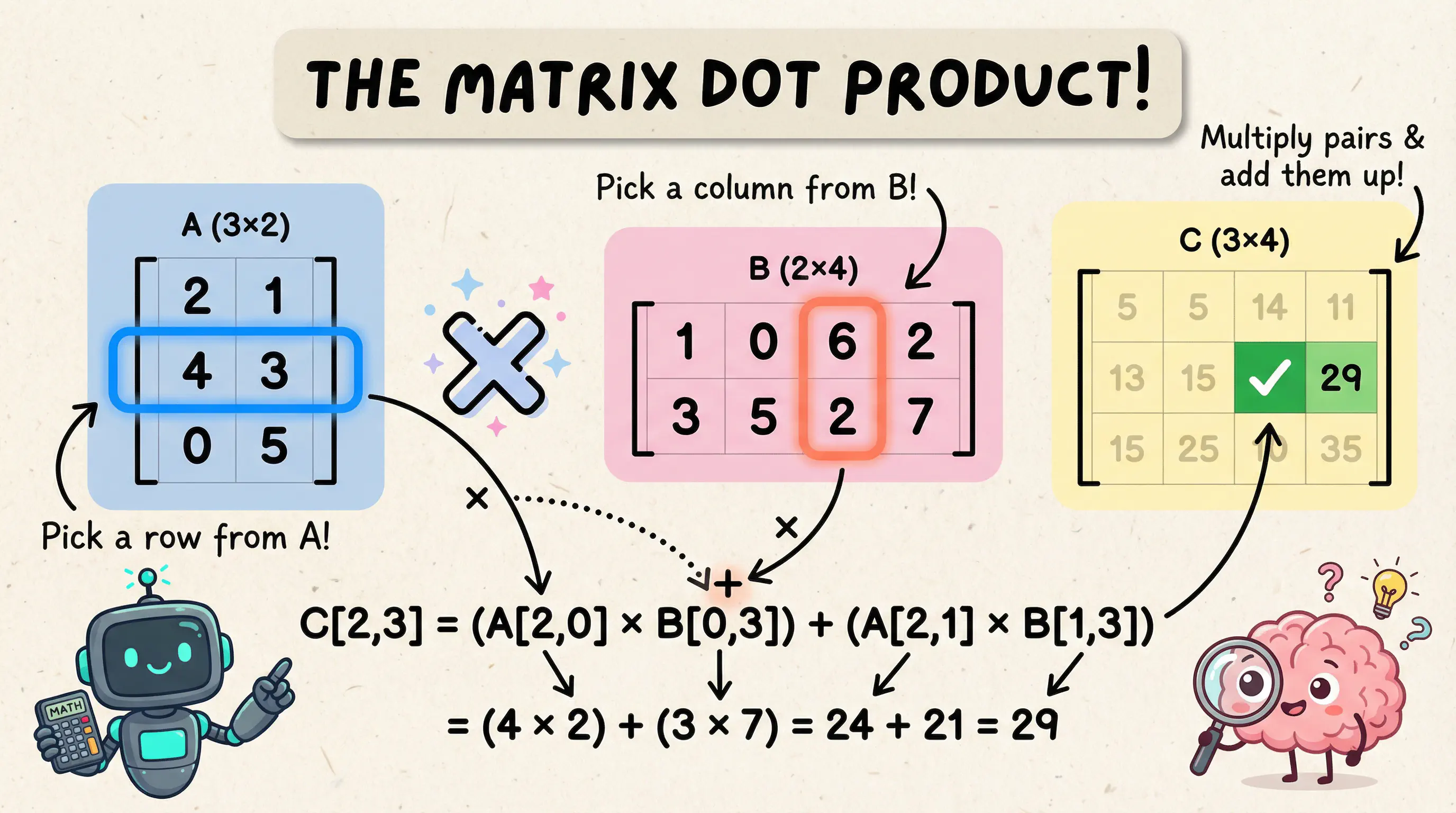
Simple enough. Now I need the core operations. The most critical one is dot (matrix multiplication):
| |
Each element in the result is the dot product of a row from the first matrix with a column from the second matrix.
I also need element-wise operations:
- add/subtract: For adjusting weights during gradient descent
- multiply: For combining gradients with activation derivatives
- transpose: Essential for backpropagation (I’ll explain why later)
- map: Apply a function to each element (for activation functions)
It’s important to note: dot() and multiply() are fundamentally different operations. dot() is matrix multiplication (rows × columns), while multiply() is element-wise multiplication (each element multiplied independently). It’s a subtle difference but an important one.
Weight & Bias Initialisation
Initialising the weights and biases of each layer may seem insignificant but actually has quite a profound effect on the network if it’s not done correctly.
Weights determine how much influence each input has on a neuron’s output. Biases, on the other hand, allow neurons to activate even when all inputs are zero - they shift the activation function left or right, giving the network more flexibility to fit the data. Think of bias as the neuron’s “baseline” tendency to fire.
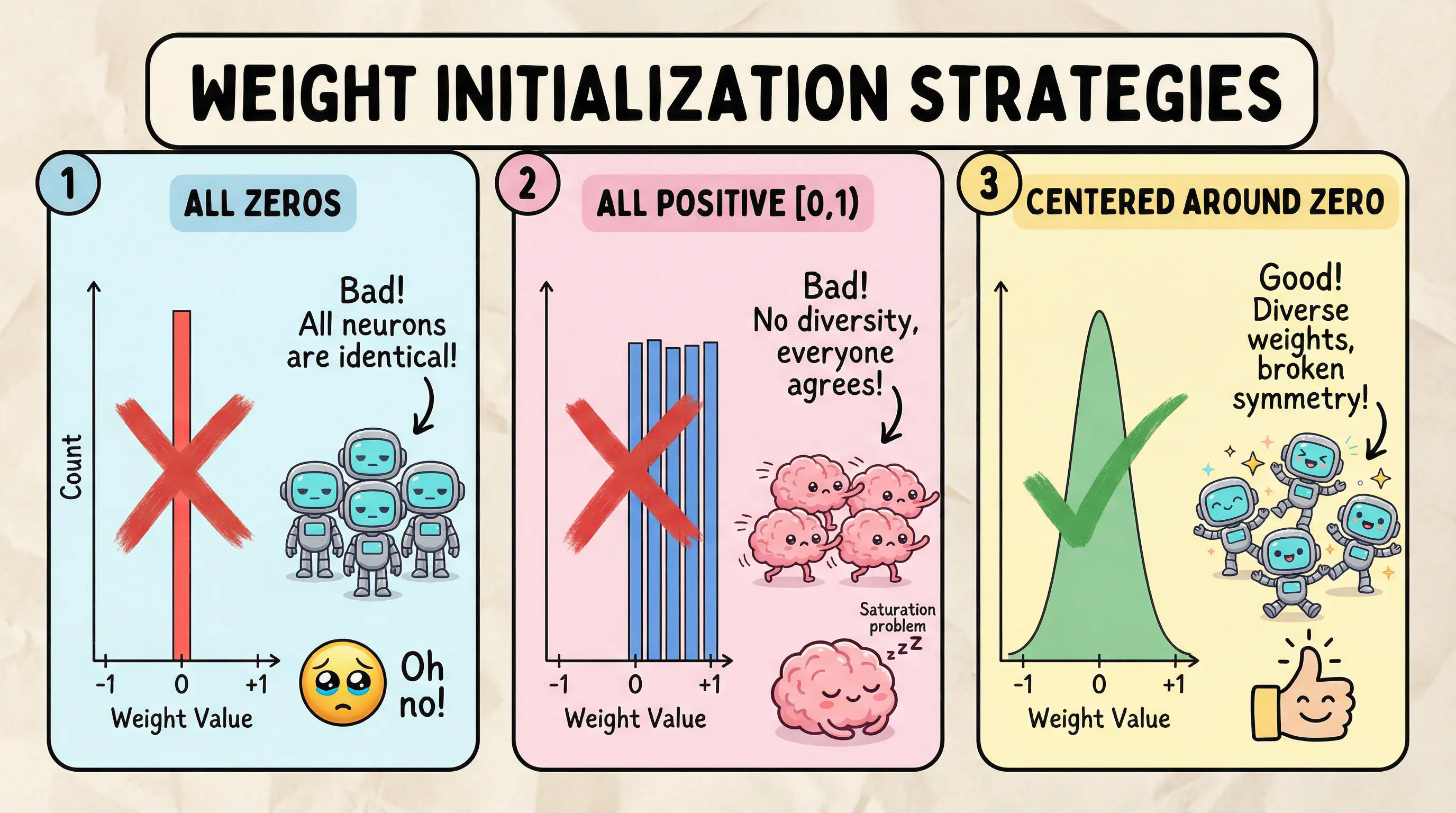
The network can’t just initialise weights to 0 - if we look at the formula applied to each layer (input × weights), multiplying by 0 gives 0. This would mean all the neurons are effectively dead. Biases, however, are typically initialised to 0, which is fine because they’re added (not multiplied) and the random weights provide enough asymmetry to break the symmetry problem.
So what should it initialise weights to? The answer is basically anything but 0, and one way to do that is using random values. By randomising each weight within a set range it provides some variation to each layer, allowing neurons to pick up on features in different ways and avoid symmetry.
| |
But wait, there’s still a problem here; all weights are positive! This causes two issues:
- Lack of diversity: All neurons respond positively to inputs, so they can’t specialise into different feature detectors
- Saturation: With sigmoid activation, all-positive weights tend to produce large sums, pushing activations into the flat regions where gradients vanish
The fix is to centre weights around 0, Rust provides the random_range function which can include negative ranges that makes this nice and easy:
| |
This works, but we can adjust the spread of these random values by applying a scale factor based on the the number of inputs: scale = (2.0 / rows).sqrt() (this is known as He initialisation). There’s a lot more research around these initialisations that I’m not going to dig into right now, this will be sufficient for what I am doing.
| |
The result of all this gives each neuron a mix of positive and negative sensitivities, enabling them to learn diverse features.
Activation Functions
Without activation functions, a neural network is just a series of linear transformations - which collapse into a single linear transformation. No matter how many layers you stack, you’re just doing linear regression.
Activation functions introduce non-linearity, which is what makes neural networks capable of learning complex patterns.
The activation function is used during the forward pass, and its derivative form is used during the backward pass.
For the implementation of these I’ll be making use of Rust Traits:
| |
Sigmoid
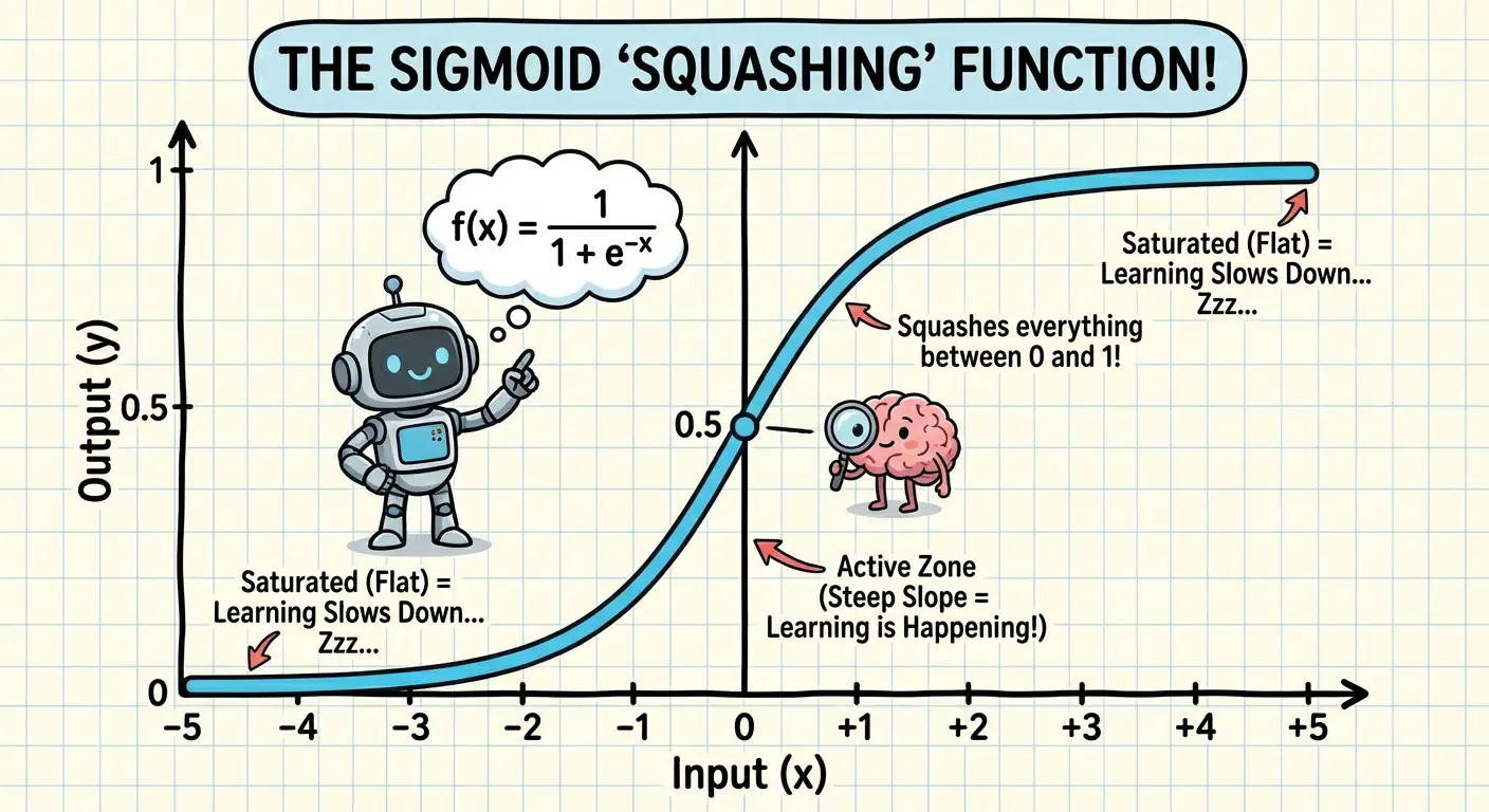
Sigmoid squashes any input into the range (0, 1):
| |
Its derivative has an interesting property:
| |
The derivative uses the activated value in its calculation. I could calculate this as part of the function but there’s an opportunity for a clever optimisation. I already calculate the activated value on the forward pass, so if I cache this, I can re-use it during the backward pass!
I apply the function to each element in the input matrix - this is where the map() implementation on the matrix comes in, and the Sigmoid implementation ends up like this:
| |
Sigmoid is great for binary classification outputs (0 or 1), but it has a problem: vanishing gradients. When inputs are very large or very small, sigmoid saturates near 0 or 1, and its derivative approaches zero. This means gradients get tiny, and learning slows to a crawl.
ReLU
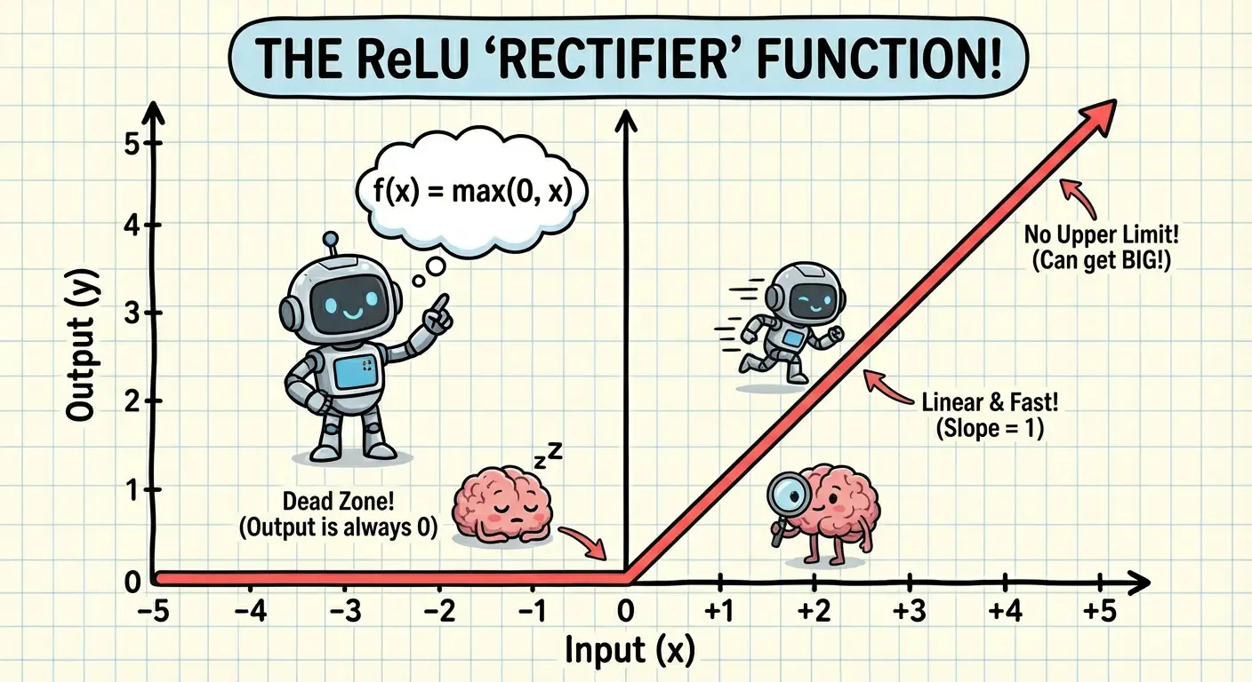
ReLU (Rectified Linear Unit) is much simpler:
| |
For positive inputs, ReLU has a constant derivative of 1, which avoids vanishing gradients.
However, ReLU has its own issue: dying neurons. If a neuron’s inputs are always negative, its output is always zero, the gradient is always zero, and it never learns. Random initialisation can trap neurons in this dead state. Something to be aware of.
Layers
A layer bundles weights, biases, and an activation function together. It also needs to cache the input and output from the forward pass, because I’ll need these during backpropagation.
| |
The forward pass is a straightforward implementation of formula:
| |
Each neuron computes: activation(input · weights + bias). For a batch of inputs, this happens in one matrix multiplication. This is where the power of using a matrix on the input comes in - I can batch multiple input features together and process them as one. In the XOR example, the entire training set is processed in a single operation; how cool is that?
Backpropagation
This is where things get interesting. Backpropagation is how the network learns - it computes gradients (how much each weight contributed to the error) and uses them to update weights.
The Chain Rule
The chain rule is the heart of backpropagation. In this case, gradients flow backward through the computational graph, and I apply the chain rule at each step.
The Backward Pass Implementation
Here’s the backward pass for a layer:
| |
Understanding the Gradient Calculations
Let me break this down:
Gradient through activation: I have
grad_output(how loss changes with respect to this layer’s output). I multiply it element-wise by the activation derivative to get the gradient before activation was applied.Weight gradient: To find how loss changes with respect to weights, I compute
inputᵀ · grad_activation. This tells me how much each weight contributed to the error.Bias gradient: Biases affect all examples in the batch, so I sum gradients across examples.
Input gradient: To propagate gradients to the previous layer, I compute
grad_activation · weightsᵀ. The transpose here “reverses” the matrix multiplication from the forward pass.Weight update: Gradient descent is simply:
weights -= learning_rate × gradient.
Why Transpose Matters
The transpose is crucial here - without it the matrix operations would be incorrect or fail. On the forward pass, the dot product of the matrix maps the input to the output shape, which must match the input of the next layer. Therefore during backpropagation the inverse must be true: transposing the matrices allows me to reshape them to fit the output back to the input.
Assembling the Network
A network is just a sequence of layers. Forward pass threads data through layers sequentially, backward pass threads gradients backward:
| |
Note the .rev() in backward pass - we iterate through layers in reverse order.
Loss Function
We need a way to measure how wrong the network’s predictions are. For this, I used Mean Squared Error (MSE). The good thing about this is that it allows the network to punish larger errors more effectively without over-correcting smaller errors, although that is also its detriment - it can be sensitive to outliers.
| |
This derivative is what kicks off backpropagation. It’s the initial grad_output that flows backward through the network.
Training Loop
With all the pieces in place, training is simple - I can add this to the Network impl:
| |
And the training loop is simply a number of iterations (epochs) over this function:
| |
Now there’s obviously some benefit to outputting and tracking more information during this process. This will allow me to plot data about the predictions over the course of the training, as well as current losses.
Serialisation and CLI
Once training is complete, it would be nice to save the resulting model. I didn’t want to get too fancy here and just used simple JSON serialisation of the network layers and their weights and biases.
For the CLI, I used the clap library to create subcommands with various parameters to allow testing different variations with relative ease, including different layer/activation combinations:
| |
Also for a bit of visual feedback the CLI outputs various plots which can help diagnose what is happening when the results aren’t quite as you expect.
I’ve glossed over this part as it was mostly just housework and not too exciting. The key point is that I can try different parameters and save/load the results, making experimentation a breeze.
What’s Next
In Part 2, I’ll actually use this network to solve problems:
- Training on OR, AND, and XOR gates
- Visualising decision boundaries to see what the network learned
- Understanding why XOR needs a hidden layer
- Testing generalisation with circle classification
I’ll also explore some of the decisions made during the implementation, and look at how things like initialisation can affect the results.
The code for this project is available on github (this links directly to the commit at the time of writing). If you’re curious about the implementation details I glossed over here, check out the full source.