In Part 1, I built a neural network from scratch in Rust, implementing matrices, activations, backpropagation, and a training loop. Now it’s time to actually use it and confirm that it works as intended.
Logic Gates
So now that I have a neural network, I need something to train it with - that is a set of inputs that I know the target output for and can easily determine correctness. Logic gates are great test problems for neural networks. They’re simple enough to train quickly, but they reveal important truths about what neural networks can and can’t do.
The data is straightforward; you have two binary inputs and a single binary output - this becomes our supervised learning data set which we can train the network with.
Let’s start with OR:
The OR Gate
OR returns 1 if either input is 1:
| Inputs | Output |
|---|---|
| [0, 0] | 0 |
| [0, 1] | 1 |
| [1, 0] | 1 |
| [1, 1] | 1 |
Training this my neuronet implementation requires a few parameters to define our input data, which columns contain our target value, what network architecture to use and finally where to save the results (I’ll just let epochs and learning rate use defaults for now):
| |
Success! I’ve solved world peace and nobody will ever go hungry again… or maybe not, but at least my neural network appears to have done something. Let’s take a look at more of the output:
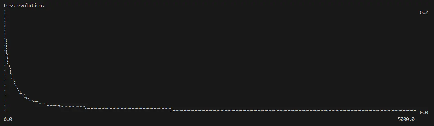
Calculated loss over number of epochs completed while training OR logic (epochs=5000, learning rate=0.6)
- Initial loss: 0.2805
- Final loss: 0.0009
- Smooth convergence curve
The final predictions were pretty good, all very close to the target:
| |
How Do the Different Patterns Learn?
I was curious to see how the different input patterns converged during the training process, and if they would do it at the same rates or different.
Taking another look at the activation formula:
output = activation(input · weights + bias)
There’s a multiplication using the input value, therefore the result of any of the 0 inputs will end up as 0 in that calculation effectively relying solely on the bias value for the activation. So this makes me think that the [1,1] input would train faster as it has the full compound impact of the weights and biases pushing in a single direction.
To test this, I added an additional plot to the command output, this plots a line for up to 4 inputs:
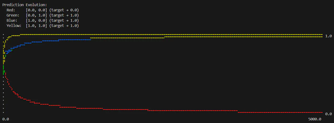
Logical OR predictions over number of epochs completed (epochs=5000, learning rate=0.6)
- [1, 1]: Fastest to 1.000 exactly
- [0, 1] and [1, 0]: Middle-tier, very similar rates to 0.9723
- [0, 0]: Slowest, down to 0.0442
Perfect! The data proves the theory; visuals are something I love as they really help tell the story of the data. Using ASCII graph plots is a little limited, and the lines get a bit confused but I’ll continue to use this to help see the results throughout different tests - it’s nice and easy to see straight off the bat without any additional processing and is fine for my personal playground (in practice I’d want some a little more robust!).
The AND Gate
Now we have OR solved, let’s take a look at the AND gate:
| Inputs | Output |
|---|---|
| [0, 0] | 0 |
| [0, 1] | 0 |
| [1, 0] | 0 |
| [1, 1] | 1 |
So we can see that for the AND logic both inputs must be 1 to produce an output of 1. Nice and simple - let’s see how it trains:
| |
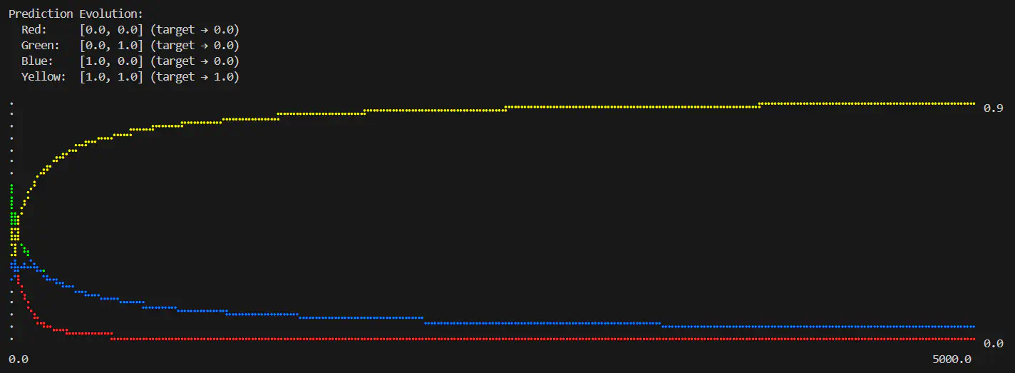
Logical AND predictions over number of epochs completed (epochs=5000, learning rate=0.6)
This is interesting, you can see for AND [0,0] very quickly reacts in a similar way to the [1,1] OR input. Additionally, it’s interesting to note that AND [1,1] input matches the convergence rate of the OR [0,0] - so it seems like a straight swap between the two.
The XOR Gate
OK, now for XOR; This was my initial goal: train a neural network to understand XOR logic. Did I do it? Let’s find out.
XOR:
| Inputs | Output |
|---|---|
| [0, 0] | 0 |
| [0, 1] | 1 |
| [1, 0] | 1 |
| [1, 1] | 0 |
| |
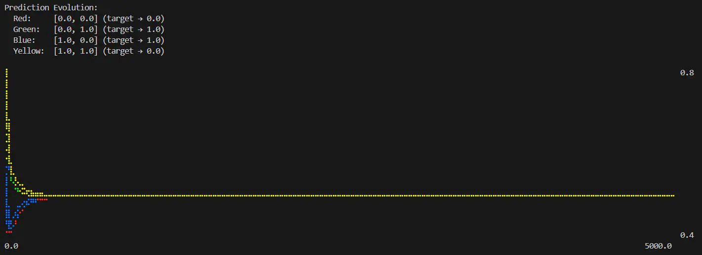
Logical XOR predictions over number of epochs completed (epochs=5000, learning rate=0.6)
That is what I’d call a failure. None of the predictions are correct, and seem to have got stuck smack in the middle. The losses don’t reduce to near 0 throughout the entire training period.
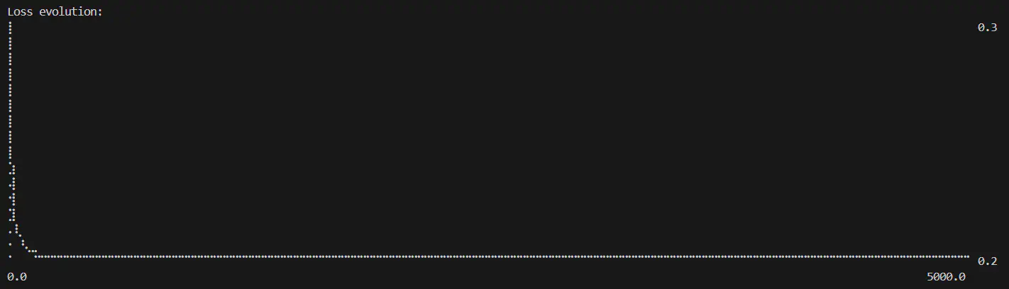
Logical XOR losses over number of epochs completed (epochs=5000, learning rate=0.6)
Why XOR Matters Historically
I mentioned in Part 1 that this was once thought impossible, it turns out that this is the reason why. In the 1960s, researchers proved that a single-layer perceptron cannot solve XOR. This contributed to growing skepticism about neural networks and played a role in the period now called the “AI winter” - a time when funding dried up because neural networks seemed fundamentally limited.
Why can’t it be solved? It’s down to being non-linearly separable. Which is actually quite a simple concept: if you visualise the truth table as a 2D grid, place chickens on the 0 values and foxes on the 1’s - now try and put in a fence to separate the foxes from chickens.
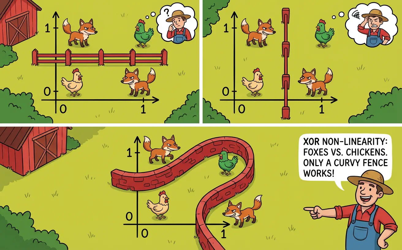
The only way to separate the foxes from the chickens is using a non-linear fence (or multiple fences)
The solution? Hidden layers. A multi-layer network can transform the input space into a new representation where XOR becomes separable.
In electronics, an XOR gate is typically built from simpler gates: XOR(a,b) = (a OR b) AND NAND(a,b). That is, “at least one input is high” AND “not both inputs are high”. The hidden layer lets the network learn these intermediate representations - one neuron can act like an OR gate, another like a NAND gate - and the output layer combines them.
Hidden Layers
The parameter I have added to allow this is the --layers argument, which so far all tests have used a single 1:sigmoid layer value. This is always in addition to an implied input layer which is determined by the input features (in this case 2 features as our binary input pairs). So we have 2 inputs into 1 neuron using sigmoid activation, and we have no further layers so that gives the final output.
For XOR we need an additional layer, so let’s try adding an extra 1:sigmoid:
| |
Logical XOR losses over number of epochs completed (layers=2:input-1:sigmoid-1:sigmoid, epochs=5000, learning rate=0.6) Logical XOR predictions over number of epochs completed (layers=2:input-1:sigmoid-1:sigmoid, epochs=5000, learning rate=0.6)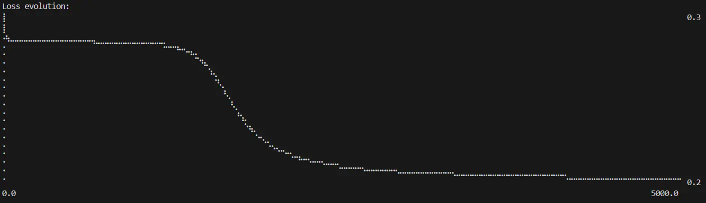
There’s some response to the additional layer, in this example at least 1 of the inputs appears to converge correctly, but the rest all end up in the same sort of limbo. Now clearly just adding an additional single neuron layer isn’t enough - let’s modify that extra layer with 1 more neuron (2:sigmoid):
| |
Wahey! This looks like a good result, the predictions are roughly where I want them - it’s not perfect but I’m not too worried about fine tuning the results just yet (I’ll have to do another post on that to stop this getting too long!).
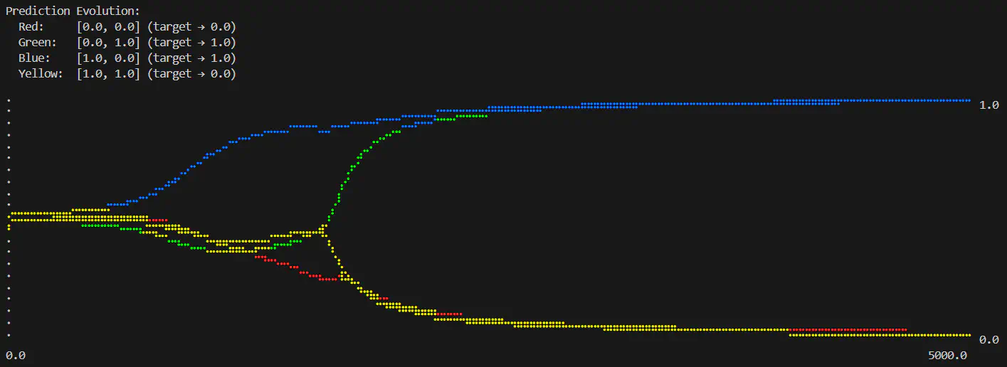
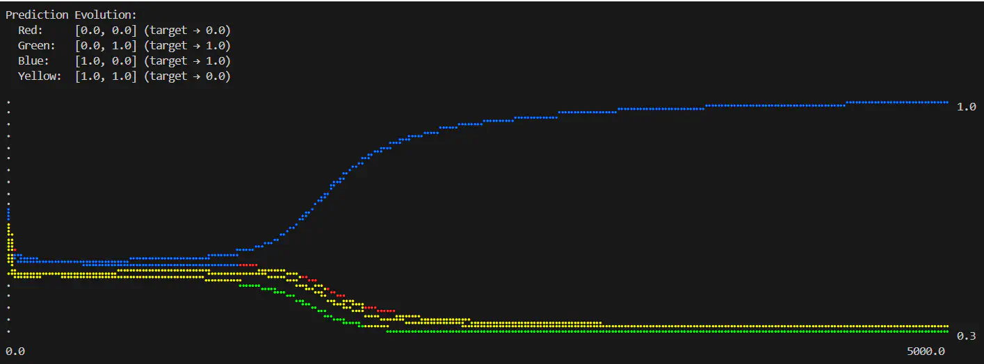
Logical XOR predictions over number of epochs completed (layers=2:input-2:sigmoid-1:sigmoid, epochs=5000, learning rate=0.6)
The convergence plots are a lot more interesting now; it actually starts off almost exactly the same as with a single neuron layer, but then there’s a sudden split where it course corrects - the weight adjustments must really ramp up there.
We can see how this initial hesitation seems to drag the loss convergence out too:
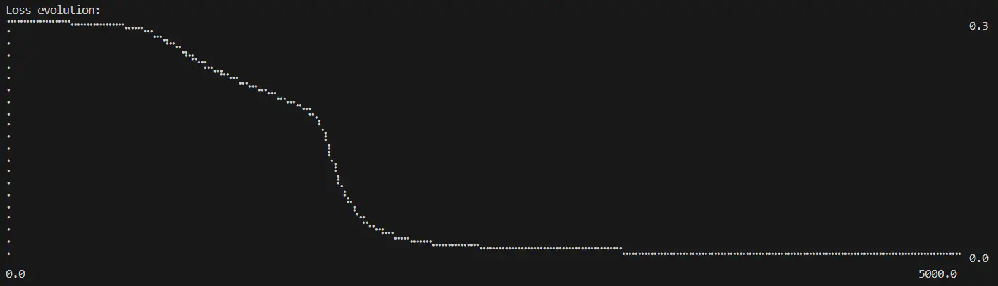
Logical XOR losses over number of epochs completed (layers=2:input-2:sigmoid-1:sigmoid, epochs=5000, learning rate=0.6)
There’s also that same sudden correction - seemingly around when the network discovers the correct OR logic. I think it’s pretty cool to see that play out. I don’t want to get too heavy on the maths at the moment so I’m not going to dig into the numbers to figure out what’s going on there just yet (maybe a future deep dive if I find the time).
Why did this work then? What does the hidden layer actually do?
With a hidden layer, each neuron can learn a different feature—just like building an XOR gate from simpler components:
- One neuron might learn “at least one input is high” (like an OR gate)
- Another might learn “not both inputs are high” (like a NAND gate)
- The output neuron combines them: when both conditions are true, output 1
It’s almost exactly how you would construct an XOR logic gate in electronics by combining outputs of other gates. And in much the same way that combining logic gates together can build complex systems like the machines we use every day, adjusting the size of the network seems to allow much more complex patterns to be evaluated.
What Does this Actually Achieve?
This is all fantastic, but how is this actually useful? I’ve got an algorithm that can take some input and predict the output - but hang on, I already had the output in order to train it… isn’t this all a big waste of time?
The logic gates are a massive simplification, but even so, when you look at all the values inbetween 0 and 1 it becomes a bit more obvious that the network has actually learned more than what I input during training - what happens if you ask it to predict the output of [0.24,0.394]?
I added the test command to try this out. It takes the saved output model from the train command and a file containing inputs (no targets this time!), this then outputs the predictions for all the inputs based on the weights and biases that we saved in the model when it was trained.
The network has been trained on a set of data, but can now tell us about data that it has never seen before! Aha! Now that seems like it could be much more useful.
Visualising Decision Boundaries
There’s a lot of numbers flying around now, but how can I see what the network has learned? For binary problems like these logic gates I can simply use the inputs as coordinates and use a colour to represent the value at each point, e.g. a gradient from black (0) to white (1). Not very complex but it should be enough for a simple demonstration.
I added the visualise command just for this, it generates a 2D grid of points across the input space of varying resolutions, runs predictions on all of them using a saved model, and displays the results as in ASCII:
| |
This generates 50x50 = 2500 predictions, showing confidence levels with gradients.
OR Decision Boundary
Logical OR decision boundary (layers=2:input-1:sigmoid, epochs=5000, learning rate=0.6)
Not the most breathtaking of images, but this shows the linear separation between 0 and 1 in the OR truth table quite well; most of the grid is bright white with a fade to black at [0,0]. It may be possible to sharpen that decision boundary by tweaking some of the parameters that it’s trained with (I’ll be doing a systematic run through of different parameters as part of what has now evolved into a series of posts).
AND Decision Boundary
This is essentially the opposite of the OR image, the only bright white section is when both inputs are high.
Logical AND decision boundary (layers=2:input-1:sigmoid, epochs=5000, learning rate=0.6)
XOR Decision Boundary
If I refer back to the foxes and the chickens, I can see what is going to happen now for XOR: I get two fences!
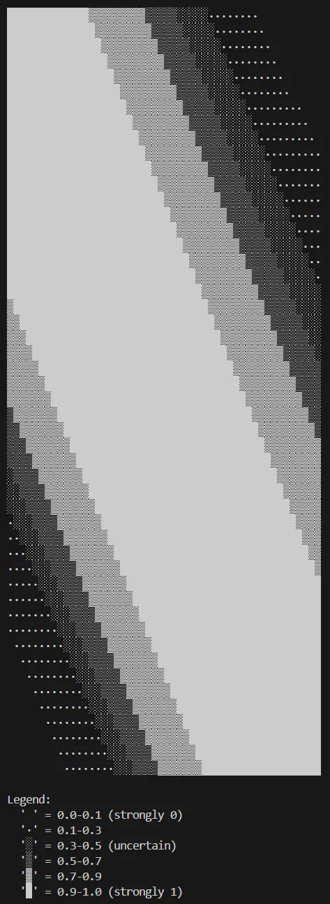
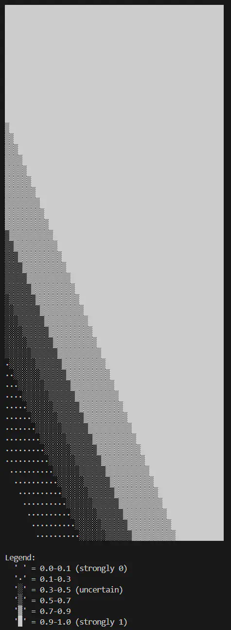
Logical XOR decision boundary (layers=2:input-2:sigmoid-1:sigmoid, epochs=5000, learning rate=0.6)
I trained on 4 points, the visualisation shows predictions for 2500 points. The network learned the concept of XOR, not just memorised the four training examples.
The gradient zones (medium brightness) show the network’s uncertainty near the boundary. At the corners, it’s confident. Near the diagonal, it’s less sure - which makes sense, since that’s where there is a transition.
This is what really defines machine learning, at no point did I actually explain the rules of the logic to the program.
It’s more like:
“Hey, here’s some values that give me these results” “Can you tell me what result I’d get for these other values?”
The network learned the pattern from 4 examples and can now apply it to any point.
Circle Classification
Now for something less straightforward to put it this all to the test a bit more. I want to train the network to identify a circle.
In order to do this, and prove the network was able to learn, I’m keeping it 2D to make use of the boundary visualisation. I’ll need some data points that represent random coordinates in the grid space, my target in this instance is a simple label that says whether the point is inside or outside the circle (I can use 1 and 0).
Generating Data
This seemed like a good fit for a Python script to generate the data:
| |
Training and Testing
| |
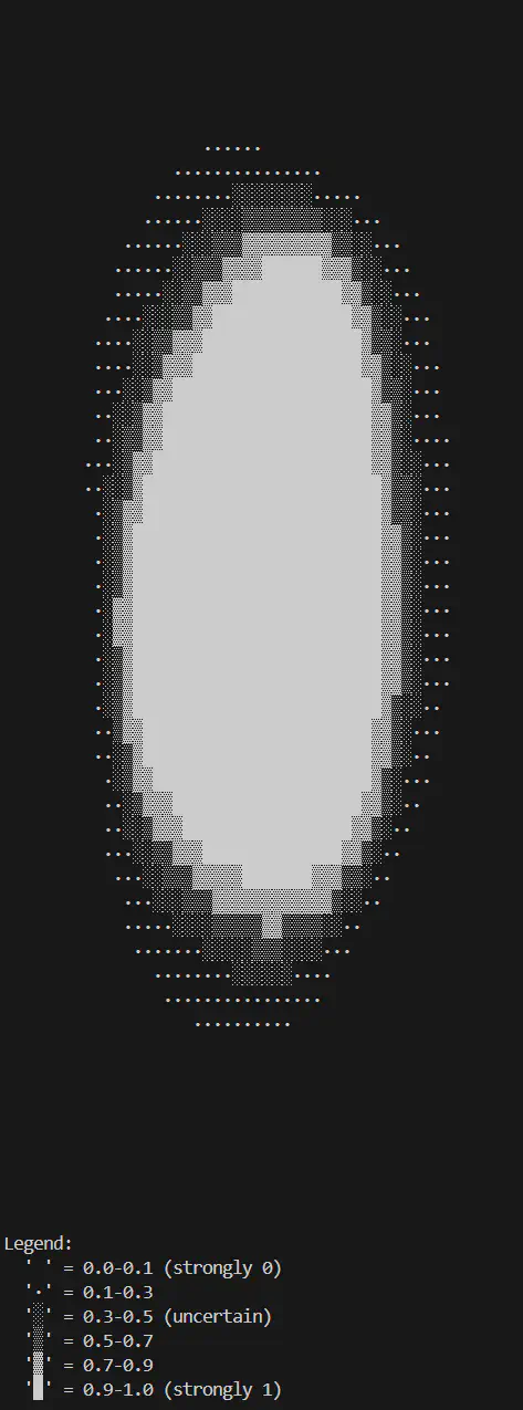
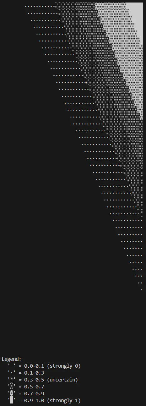
Circle classification decision boundary (layers=2:input-4:sigmoid-1:sigmoid, epochs=5000, learning rate=4.0)
Great success, the visualisation shows a roughly circular boundary in the middle of the grid space. Not perfect, and not helped by my ASCII characters being rectangular - but clearly showing that the network learned the general pattern.
I did have to trial-and-error a few parameters to get a stable result hence the increased learning rate and neuron count on the hidden layer - this is a much more complex problem than any of the other examples so far.
- Training data: 100 random points labeled inside/outside
- The targets represent what “circleness” looks like
- Network learns the concept: “distance from centre < radius”
- Can then apply this to any point in the space
The network doesn’t memorise the 100 points. It learns to:
- Interpolate: Predict points between training examples
- Generalise: Apply the concept to completely new data
- Extrapolate: Predict across the entire input space
The decision boundary visualisation proves this - I trained on just 100 points but can see predictions for 2500 grid points.
What’s Next
So far it’s all been quite trivial, but still it’s really been quite fun seeing how this all works. I’m a long way off training a Large Language Model at this stage, but I can see how this would fit into training on natural language inputs to produce natural language outputs.
There are some things that I’d like to continue to visit back in this series:
- Optimisers: I’ve used vanilla gradient descent, but there are alternatives to optimise this
- Regularisation: L2 penalty, dropout, batch normalisation prevent overfitting
- Convolutional layers: Specialised for image data
- Recurrent layers: Specialised for sequential data
- Attention mechanisms: The foundation of transformers
All of these are built on the same fundamentals I have implemented here: forward passes, backpropagation, gradient descent - so it can’t be too hard!
Try It Yourself
The code for this project is available at GitHub.