In Part 1, I built a neural network from scratch in Rust. Now it’s time to actually use it - but not just to solve problems. I want to understand why certain choices matter, and what happens when things go wrong.
This is the first in a series of posts I hope to continue between other projects, documenting experiments with my neural network implementation and understanding how it works, and how it can be improved. The goal here is to continue to develop and understand the implementation by building it myself - so the experimentation will be done with that idea in mind.
Experimentation

For each experiment, I’ll follow a consistent structure:
- What am I trying to learn?
- What do I expect to happen, and why?
- Controlled experiment with one variable changing
- What actually happened
- What does this tell me?
This might look a bit like your traditional scientific method and seem overly formal for me mucking about, but one of the many things life has taught me is that repeatability is paramount to true understanding. It helps catch assumptions and makes it easier to spot when results contradict expectations - if I don’t know what exactly caused a result, how can I possibly know for sure how to get that result again? (I spent a lot of time during the COVID lockdown making pizza dough and the same theory applied there!).

The scientific method applies everywhere - even pizza dough
CLI Improvements
My initial ASCII plots were quite limited - so I had a bit of a play around to try and make them a little better; it didn’t really matter what I did, they were a bit naff. The CLI instead no longer outputs plots directly, instead the raw data from a training run is stored according to the options specified; this data can then be analysed more effectively by other tools. That being said, I did include an animated visualisation of boundary evolution… just because I thought it was pretty cool to see.
I have extended the CLI to include an option to provide an initial seed to the train command (this is also saved in the model metadata). This should enable the training to be run again with the exact same weight initialisation for reproduction. This can aid with seeing how changes to the implementation have affected results, as well as investigating issues with specific test runs.
The final thing to note, many of these experimentations require multiple training runs - the randomisation of initial weights leads to different results each time. Therefore, in addition to providing a fixed seed, it makes sense to add an option to automate multiple runs. So There’s now an iteration option for training too.
Establishing Baselines
Before I can measure anything, I need to know where I’m starting from; you can’t measure your height if you don’t know where the ground is. A baseline gives me a reference point for all future experiments. I’ll set a couple of baselines based on my initial training problems - XOR and circle classification.
I’ll first gather some data, and then do a bit more of a deep dive into actually analysing this data which is something I haven’t really done since my uni days so I’m a little rusty! I’ll take the opportunity to use Python for this, it is pretty good for data analysis using tools like pandas and NumPy.
Baseline 1: XOR Problem
XOR seems to be like the “hello world” of neural networks - four quite simple input patterns, it’s non-linearly separable, and it requires at least one hidden layer. If the network can’t solve XOR reliably, something fundamental must be broken. This seems like a good baseline to start with.
Setup:
- Architecture: 2→4:sigmoid→1:sigmoid
- Learning rate: 1.0
- Epochs: 2000
- 10 runs with different random weight initialisations
I’m keeping the parameters fairly simple for now, all Sigmoid acivation, the learning rate and epochs are more or less just numbers plucked out of thin air for now - I verified that the training was able to at least complete successfully. I will explore these parameters individually once I have this baseline data.
Results:
With a sprinkling of javascript and some magic from Claude, my original ASCII plots are replaced with:
Training Analysis
Here we can see that over the course of training the losses are reduced to near 0 in a smooth curve. The predictions of the model as the training progressed show a clear separation of classifications emerging, which is further demonstrated in the (now beautifully animated) boundary decision visualisation.
It may not be the cleanest of results - the loss training curves seem quite inconsistent between iterations and I’m not totally sure how much that matters. But the main point is that I now have a great visual reference to easily compare to when tuning hyperparameters.
Baseline 2: Circle Classification
My next baseline is something a little more that just XOR: circle classification. I already demonstrated the ability for my network to be trained on identifying points that fall within the circle data in a previous post, and how that can be used to infer additional points that are / are not within the defined circle.
Setup:
- Generate data: 100 training samples, 1000 test samples
- Circle centre: (0.5, 0.5), radius: 0.3
- Architecture: 2→4:sigmoid→1:sigmoid
- Learning rate: 4.0
- Epochs: 3000
- 10 runs with different random weight initialisations
Very similar setup to the XOR baseline to start with - although I have increased the learning rate and epochs a touch just to get a more stable result to start me off.
Results:
Training Analysis
The results actually look quite good in the boundary visualisation - this was trained on just a small subset of the data that represents the shape yet, it’s able to clearly define a fairly good circle. All the loss curves are quite smooth, but the prediction evolution plots compared to the logic gates are a little more chaotic due to the larger number of inputs.
Analysing the Baseline Data
This is something I’m going to need to do not just for these baselines, but for results of experimentation too. I need to be able to empirically state what has changed in the results in a succinct manner in order to make informed decisions based on those results.
To start with analysing the baselines I need to think about what kind of information would be useful to know, I think for now I’ve settled on these data points:
- Mean loss and standard deviation
- Accuracy and accuracy variance
- Convergence rate
What can these tell me? The final loss tells me if the training has actually converged or not, does it produce the correct results? The mean and standard deviation across different iterations will then indicate how reliable that result is, is that a rough idea of what result I would get? Or is it just a middle of the road but there’s a chance it’s nowhere near?
Accuracy numbers will perform a similar function, except these will tell me how correct the result is relative to target input. This then combines with the loss variance to determine not only how likely I am to get the same results, but also how likely those results are to be accurate.
Finally, convergence rate is something that I think would be useful to see in order to determine how best to tune hyperparameters for more efficient training. The end results might be the same but if convergence can be sped up then ultimately it means that training uses less computation and therefore lower energy/cost/human sacrifice etc. I can measure this with the number of epochs to reach a defined convergence threshold.
The Analysis Script
To facilitate the analysis I’ve written Python script using pandas to analyse the raw training data. It’s quite a simple workflow: load all iteration data, aggregate across runs, and export for visualisation (that’s the output that is used for what you see here).
The core of it is this simple function for calculating mean and standard deviation at each epoch:
| |
And for measuring convergence speed - finding the first epoch where each iteration drops below a threshold:
| |
The script exports JSON files that feed into the visualisations below. Nothing fancy, but it gives me consistent, reproducible analysis across all my experiments. I really like how easy pandas made this.
Understanding the Metrics
Mean and Standard Deviation across iterations tells me both the typical result and how much variation there is between runs. What’s interesting is how the relative spread changes during training. At the start, all runs have similar loss (around 0.25 for XOR) because the untrained network predicts roughly 0.5 for everything. But as training progresses, some runs find good solutions faster than others, and the spread increases relative to the shrinking mean.
This is why looking at standard deviation alone can be misleading - a std of 0.003 sounds tiny, but if your mean is also 0.003, that’s huge variability. The ratio of std to mean (coefficient of variation) is more meaningful.
Epochs to Threshold measures how quickly training converges. I’m using loss < 0.1 because it’s roughly where the network starts producing useful results for these problems. The mean tells me typical convergence speed; the std tells me how consistent that speed is across different random initialisations.
Visualising Training Stability
Here’s what the XOR training looks like when we aggregate across all 10 runs:
The shaded band shows ±1 standard deviation around the mean. You can see the band is relatively narrow at the start (all runs similarly bad) and stays fairly consistent throughout (although maybe a little flabby due to one iteration stalling for longer) - suggesting the training is reasonably stable across different weight initialisations.
For circle classification:
Similar pattern, though the training takes longer and the final loss is slightly higher - as expected for a more complex problem.
What the Baselines Tell Me
Now for the actual numbers. Here’s what the analysis script produced:
XOR Results:
All 10 runs converged successfully, reaching loss < 0.1 in an average of 895 epochs (with quite a bit of variance - std of 311). The final loss of 0.0035 ± 0.0026 tells me the network is learning XOR reliably, though some runs end up notably better than others. More importantly, 100% test accuracy - the network correctly classifies all four XOR patterns every single time.
Circle Results:
Again, 100% convergence rate, but taking longer (1445 epochs on average) and settling at a higher final loss (0.0145 ± 0.0049). This makes sense - the circle problem is more complex than XOR’s four discrete points, so there’s more to learn and more room for variation.
The real validation comes from test accuracy: 95% ± 1% on 1000 held-out test points. The network was trained on just 100 samples but generalises well to unseen data - it’s genuinely learned the circular decision boundary rather than just memorising the training examples.
These Numbers as Controls:
These baselines now serve as my reference point. When I tweak the learning rate, change the architecture, or try different activation functions, I can compare results against these numbers. If XOR suddenly takes 2000 epochs to converge or the circle’s final loss jumps to 0.05, I’ll know something has changed - and more importantly, I’ll be able to quantify how much it changed.
Learning Rate Sensitivity
With baselines established, let’s investigate the first hyperparameter: the learning rate. I’ve already seen when setting the baselines that there is some difference here so I’ll be testing this independently against both XOR and circle problems.
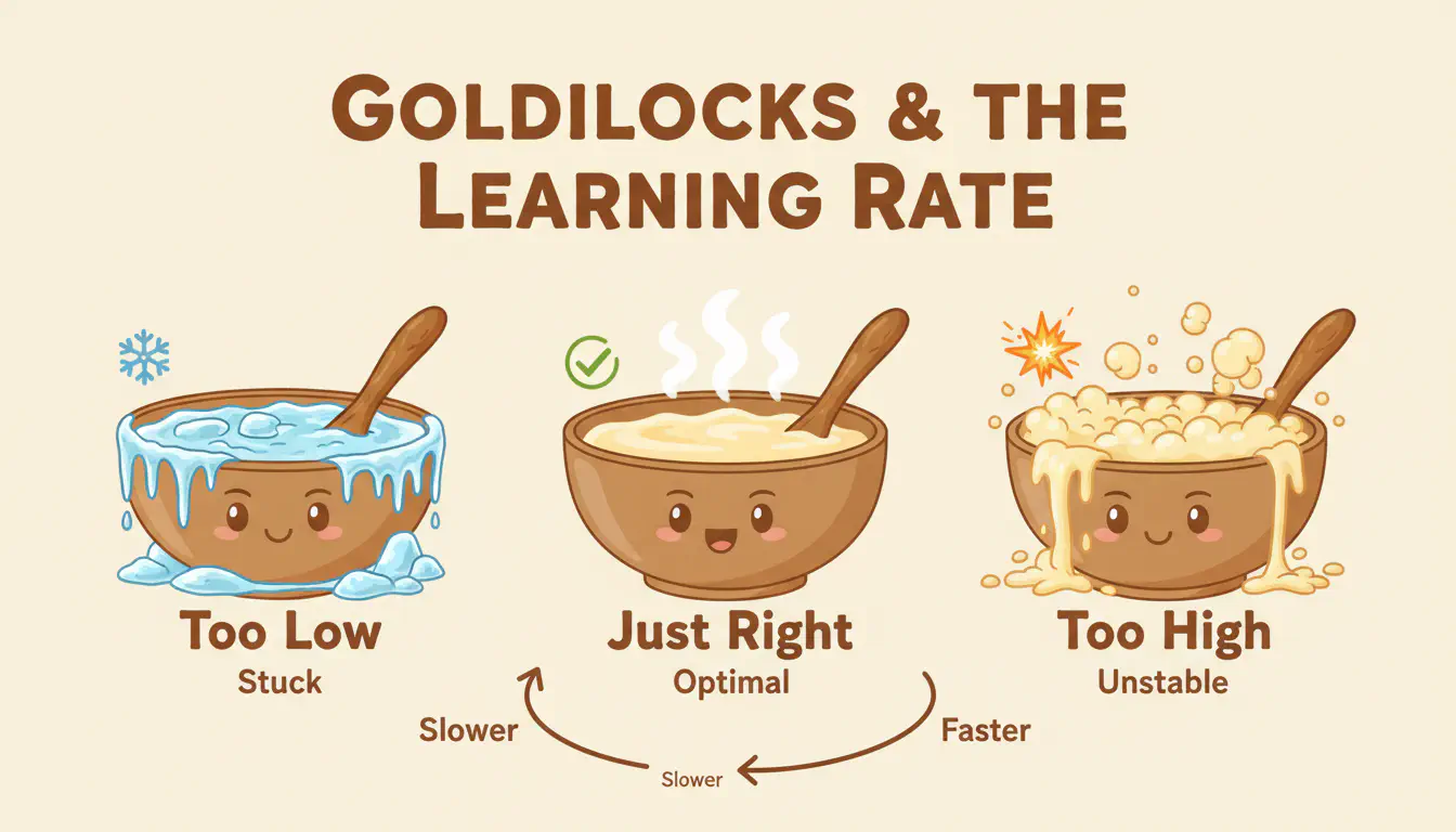
Hypothesis
I expect there’s a sort of “Goldilocks zone” - too low and training stalls, too high and it overshoots. When setting up the baselines, I already noticed that XOR worked fine with LR 1.0 and 2000 epochs. Circle classification, though? I had to bump it up to LR 4.0 and 3000 epochs just to get something to work with.
That was unscientific trial-and-error at the time - I was just trying to get the baselines working. But it highlighted the fact that different problems have differnt characterstics that appear to require different setups that aren’t directly trasnferrable.
Let’s find out properly.
Finding the learning rate sweet spot
Setup
I tested both problems with the same range of learning rates, keeping everything else consistent with their respective baselines:
| XOR | Circle | |
|---|---|---|
| Architecture | 2→4→1 | 2→4→1 |
| Activation | sigmoid | sigmoid |
| Epochs | 2000 | 3000 |
| Iterations | 5 per LR | 5 per LR |
Learning rates tested: 0.01, 0.1, 0.5, 5.0, 10.0, 25.0, 50.0
That’s a wide range - from barely adjusting anything to potentially overdoing it an alrming amount. Let’s see what happens.
Results
XOR:
Circle:
The Goldilocks Zone: Higher Than Expected
The first thing that jumps out: the sweet spot is way higher than I expected.
I assumed LR 1.0 was reasonable a reasonable start, that’s where I started for the baselines. But looking at the data - the real sweet spot is far beyond that. For XOR it lookds pretty good anywhere between 1.0 to 25.0 where it starts to twitch; Circle is a little tighter as it doesn’t become stable as low but in these tests somewhere between 5.0 to 20.0 looks good. At LR 10.0, XOR converges to a loss of 0.0001, orders of magnitude better than the baseline. I was being far too conservative with my baslines rates!
At the low end, LR 0.01 and 0.1 completely fail for both problems. The loss curves are essentially flat lines - the network outputs roughly 0.5 for everything and never escapes. This isn’t slow learning; it’s no learning at all.
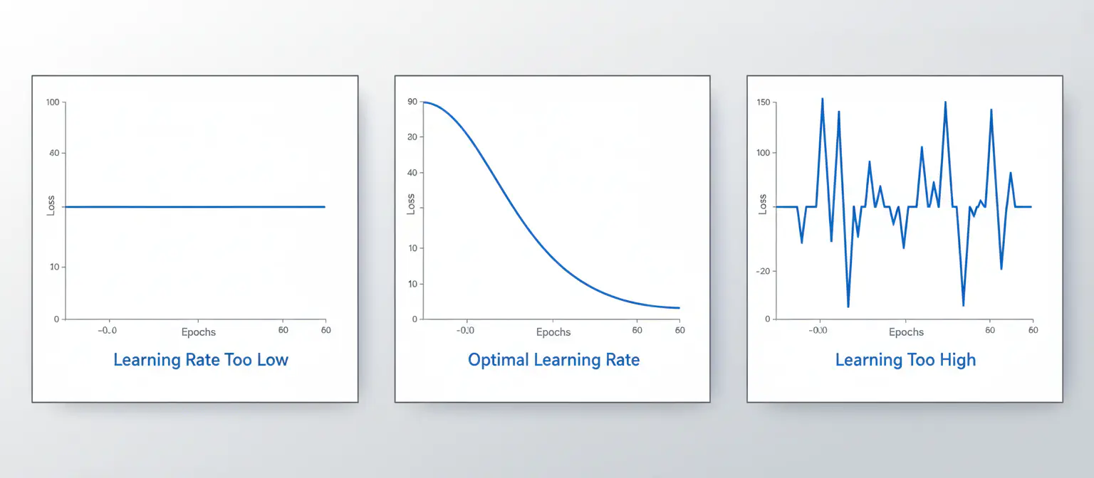
The three failure modes: stuck, converging, and unstable
Looking at LR 0.5, for XOR, it’s borderline - 4 out of 5 runs converged. For circle classification, it completely fails - 0 out of 5 converged. Same learning rate, same architecture, completely different outcomes.
The ideal Learning Rate isn’t universal. It shifts depending on the problem.
The circle problem needs more aggressive learning rates to get moving. Looking at the data, both problems share the same sweet spot at the high end (5.0-20.0 works for both), but the circle’s lower boundary is higher. What’s merely “borderline” for XOR is “completely stuck” for circle.
Why might this be? Circle classification has 100 training samples versus XOR’s 4. With more data points, each gradient update averages over more samples, this could be potentially smoothing out the signal. A higher learning rate might therefore be needed to compensate for that.
But What About More Epochs?
An obvious question: could I have made LR 0.1 work by just running more epochs? Looking at those flat loss curves, my initial assumption was no - the network appears stuck, not slow.
But assumptions should be tested. So I ran LR 0.1 and 0.01 for 2,000,000 epochs instead of 2,000. And… they converged. Both of them.
It turns out those “flat” curves weren’t flat forever - they just needed much longer to get moving. The network wasn’t stuck; it was just making progress too slowly for 2,000 epochs to show.
This raises an interesting question: if low learning rate plus high epochs can eventually work, what’s the trade-off? Is there any reason to prefer one over the other?
All three configurations reach roughly the same final loss (~0.0001 or better). So yes, you can compensate for a low learning rate with more epochs. But look at the epochs-to-threshold column: LR 0.1 needs 35x more epochs than LR 10 to cross the 0.1 threshold. LR 0.01 needs 260x more.
The Trade-off
Computation time: 2 million epochs takes time. On my machine, the LR 0.01 run took noticeably longer than the LR 10 run. For a simple problem like XOR this is just seconds versus milliseconds, but scale that up to a real problem and it would start to really matter.
Final quality: Interestingly, all three reached similar final losses. The low learning rate runs don’t necessarily produce better results - they just take longer to get there.
Stability: Higher learning rates can be unstable (remember LR 50 only converged 3/5 times). Lower learning rates are more stable but slower. There will be times where you’d deliberately choose a lower learning rate and more epochs to avoid this instability.
Key Takeaways
Baselines matter. Without the data to say that XOR converges in ~900 epochs with LR 1.0 and achieves 100% accuracy, I wouldn’t truly have been able to say that LR 5.0-25.0 converges faster and more reliably. The baseline provides context for interpreting results, and this is true for any experiment that involves changing any variable.
The ideal learning rate may not be what you’d expect. I assumed LR 1.0 was reasonable - turns out 5.0-25.0 works much better in these cases. That may not (probably won’t) apply to a different training set, or even network architecture. If there’s a different loss function or other optmisation involved it would likely also alter results. So establishing reliable hyperparameters for a particular training setup is an important first step.
Random initialisation creates variance. Running a single training run can be misleading. LR 0.5 would have looked either perfect or broken depending on which seed I happened to use. Multiple runs reveal the true picture of stability.
Failure modes are binary, not gradual. The network either learns or it doesn’t. There’s no graceful degradation between “converges well” and “doesn’t converge at all”.
Learning rate and epochs trade off. Low LR + high epochs can match high LR + low epochs in final quality, but takes orders of magnitude longer. For efficiency, prefer higher learning rates - but if I’m hitting instability, running longer with a lower rate is a valid fallback.
What’s Next
With an idea of what effect the training paramaters have, I’m ready to explore architecture choices:
- Does depth or width matter more for learning complex patterns?
- Sigmoid and ReLU; different activation functions?
- Alternative loss measuerements?
The code for these experiments is available at github.com/lordmoocow/neuronet.